A comprehensive computational model of facilitated diffusion in prokaryotes

Abstract

1 INTRODUCTION

Originally, it was believed that transcription factors (TFs) find their target sites only through 3D diffusion and the association rate would follow the Smoluchowski limit. Riggs et al. were the first to observe that the rate at which the lac repressor locates its target site is much faster than the rate predicted by the Smoluchowski limit and hypothesized that a different mechanism was involved in this process (Riggs et al., 1970).

In their seminal work, von Hippel et al. (Berg et al., 1981; Winter et al., 1981) thoroughly investigated this process from both a theoretical and experimental perspective and concluded that TF molecules use the facilitated diffusion mechanism to locate their target sites. This facilitated diffusion mechanism assumes a combination between 3D diffusion in the cytoplasm and an 1D random walk on the DNA. This leads to reduction of dimensionality in the search process and, consequently, speeds up the search. In addition, three main types of movements on the DNA were proposed: (i) sliding, (ii) hopping and (iii) jumping (Berg et al., 1981). Sliding and hopping are both mechanisms of 1D random walk, but the difference between them is that during hopping the molecules lose contact with the DNA, whereas during sliding the molecules keep contact with the DNA. On the other hand, jumping is a mechanism which assumes that the molecules do not only lose contact with the DNA for a short time interval (as in the case of hopping), but they completely release into the cytoplasm where they spend a longer time until they bind to the DNA uncorrelated with respect to the unbinding position.

The existence of the 1D random walk in vivo was recently confirmed by (Elf et al., 2007). The authors of that study used fluorescent lac repressor tetrameters and visualize their movement in a live Escherichia coli cell, confirming that the molecules spend 90% of the time bound to the DNA.

There are still missing pieces in our understanding of the facilitated diffusion mechanism. One approach to address these questions consists of building a computational tool able to simulate the relevant molecules in a cell and the entire DNA sequence. This type of approach can address several questions, e.g. how crowding can influence the search process at genome-wide level, in a dynamical context (Chu et al., 2009) and not as static barriers (Li et al., 2009). In addition, one could investigate systems with real affinity landscapes, which is not possible through analytical tools (Berg et al., 1981).

In this article, we present a computational model for stochastic simulation of the search process of TFs for their target sites on the DNA. The model considers each TF molecule as an independent object, which can move freely in the bacterial cytoplasm, but which also can bind to the DNA and perform an 1D random walk. The DNA molecule is modelled as a string of nucleotides, which leads to specific affinity between a TF molecule and DNA at the position where the molecule is bound. We also go through the literature and systematically infer each microscopic parameter of the model from experimentally macroscopic measurements.

Finally, we developed an implementation of the proposed model, which is available in Zabet and Adryan (2012).

2 MODEL

One strategy to stochastically model the TF search process for their target sites consists of designing a hybrid system combining agent-based modelling and stochastic simulation techniques (Gillespie, 1977). In this model, each TF molecule is represented as an agent able to perform certain actions and the DNA molecule as a string of the nucleotides: a, t, c or g. The model can assume reflecting boundaries (TFs that reach the boundary can only go back), periodic boundaries (the DNA is assumed to be in a closed loop) or absorbing boundaries (TFs that reach the boundary will unbind from the DNA).

In this setting, the TF molecules can be either free in the cytoplasm or bound on the DNA at a certain position. A free TF molecule has only one action available, namely, to bind to the DNA.

2.1 Binding event

We assume that the bacterial cytoplasm is a perfectly mixed reservoir from where the free TF molecules bind to the DNA. The 3D diffusion of TF molecules in the cytoplasm is not modelled explicitly, but rather, the molecules that are free in the cytoplasm have a certain association rate to the DNA. To simulate 3D diffusion we use the Direct Method implementation of Gillespie Algorithm (Gillespie, 1977) which generates a statistically correct trajectory of the Master Equation.

The rate at which a TF molecule of species x will bind to the DNA is computed as

(1)

where k^assoc_x is the reaction probability rate constant for species x, TF^free_x the number of free TF molecules of species x and the last fraction ( A_x^current/A_x^max) is the proportion of free positions where a molecule can bind. A comprehensive list of all parameters used in this article can be found in the Supplementary Material.

Note, that after each 1D move, the number of available positions on the DNA for a TF to bind can change and, consequently, the association rate needs to be updated often. An approximate system would consider that the binding of TF molecules is affected by occupancy, but the update is performed only when a molecule binds/unbinds and not when any other event (sliding or hopping) would lead to change in the number of available binding sites on the DNA. In the Supplementary Material, we show that the difference between this approximation and the exact system is negligible and, thus, one can use this approximate system to increase simulation speed.

When a molecule binds to the DNA it will occupy a number of consecutive base pairs on the DNA and no other molecule will be able to bind to the DNA at that position. The size on the DNA of each TF molecule is computed as the sum of the number of base pairs of the DNA binding motif, the number of obstructed base pairs on the left side of the molecule and the number of obstructed base pairs on the right side (Fig. 1).

(2)

Note that this feature (TF can cover base pairs to the left or to the right side of the DNA binding motif) has not been considered in this type of simulations, but is biologically plausible.

Fig. 1.

Open in new tabDownload slide

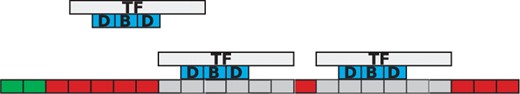
TF binding to the DNA. TF molecules bind to the DNA and mark several nucleotides as covered (grey) on: the DNA binding motif (3 bp in our example), the obstructed left side (1 bp) and the obstructed right side (2 bp). Volume exclusion is implemented, in the sense that two TF molecules cannot cover the same base pair on the DNA. The green positions on the DNA mark the positions where the free TF molecule can bind.

We mark all base pairs covered by the TF molecule as being unavailable, but we record the left-most base pair covered by the TF molecule as the position at which a TF molecule is bound to the DNA. This does not affect the results in any way, but is just a choice of internal representation of the binding.

In addition, previous simulators did not take into account TF orientation on the DNA (Barnes and Chu, 2010; Chu et al., 2009). The orientation of TFs affects the affinity of the TF for a specific position on the DNA, i.e. a molecule bound in one orientation can have a totally different affinity compared with being bound in the opposite orientation at the same position.

Finally, since transcription and translation are co-localized in prokaryotic systems, a TF molecule has a higher probability to bind initially near the DNA region where it was released, and if the target site is within a sliding length distance, the entire search process can be reduced to one sliding step. We consider the possibility of an initial binding region on the DNA in our model, in the sense that each TF molecule has a user-specified probability to bind for the first time within the user-defined region on the DNA, but only if there are free spots in that region.

2.1.1 Implementation of the binding event

Barnes and Chu (2010) observed that, in the case of crowded DNA, locating a free position on the DNA where TF molecules can bind can be a bottleneck. In the Supplementary Material, we present a new method to significantly enhance the simulation speed. This method assumes the creation and maintenance of an array list of boolean values for each TF species (x), which specifies whether a TF molecule of type x is allowed to bind at position j, A[x][j]. This has the purpose to eliminate the need to check if sufficient nucleotides (TF^size_x) in the right side of the selected position are not covered by other molecules.

Furthermore, to increase the speed of locating a position, we store the current number of free positions for each species, A_x^current, and when we look for a free position we draw a random number z in the interval [0, A_x^current) which will represent the z-th available position on the DNA. This method guarantees that a free position is found using only one random number, which represents a significant enhancement of the simulation speed. To further increase the search speed from M/2 to ⁠, we keep total counts of available positions in a different array (see Supplementary Material).

2.2 TF affinity for DNA

Once bound to the DNA, TF molecules will spend a certain time bound to a position until they make any type of movement. The time spent at any position on the DNA is determined based on the binding energy between the molecule DNA binding domain and the sequence under the molecule. The average waiting time at a position is given by (Gerland et al., 2002)

(3)

where x represents the TF species, j is the position on the DNA, τ_x⁰ is the average waiting time when bound specifically and E_x^j is the binding energy at position j. Note that the τ_x⁰ term is similar to the τ₀exp(E_ns) term in Gerland et al. (2002). The binding energies are measured in β⁻¹=K_BT (where K_B is the Boltzmann constant and T the temperature), which will leave just the value of the binding energy in the exponential term.

To reduce memory usage, we will break the TF species into two classes: (i) non-cognate TFs and (ii) cognate TFs. The cognate ones are the TFs that are of interest and that we can follow, whereas the non-cognate ones main purpose is to simulate the ‘other’ proteins on the DNA, which might interfere with the search process of the cognate TFs. For efficiency reasons, we pre-calculate the affinities of each TF species, both cognate and non-cognate, and store them in individual arrays. The non-cognate binding energy is randomly generated using a Gaussian distribution with the mean and variance provided as inputs for each non-cognate species.

The binding energy of cognate TFs is computed using two techniques: (i) mismatch energy (Gerland et al., 2002) and (ii) position frequency matrix (PFM; Berg and von Hippel, 1987; Stormo, 2000). In both scenarios, we assume that each position in the DNA binding motif is approximately independent and additive (Berg and von Hippel, 1987; Gerland et al., 2002; Stormo, 2000).

First, in the case where there is a single high-affinity binding site, one can use the mismatch energy approach, which assumes that for each mismatch between the consensus S_x for species x and current DNA position, the binding energy is penalized by a fixed value called the mismatch energy:

(4)

where L is the length of the motif and ε_x^j(k) is the mismatch penalty at position k. The mismatch penalty is equal to ε_x^j(k)=0 if S_x^k=DNA^j+k and ε_x^j(k)=ε_x^* otherwise. It was estimated that ε_x^*∈[1, 3] K_BT (Gerland et al., 2002) and, in our simulations, we will consider that ε_x^*=2· K_BT. For example, if the binding motif is atcg and between positions j and j+4 on the DNA we have the sequence acct, then E_x^j=ε_x^*×(0+1+0+1)=2·ε_x^*. Note that if there is a match between the nucleotide of the motif sequence and the one of the DNA sequence we put a value of 0 whereas for a mismatch we put a value of ε_x^*.

Second, for multiple high-affinity binding sites (experimentally determined using methods such as ChIP, SELEX and PBM) we will use the PFM. Instead of penalizing when there is a mismatch, the PFM approach has a weighted mismatch which penalizes the energy by

(5)

If at position (j+k) on the DNA we have nucleotide x, then the number of occurrences of this nucleotide at position k in all known high-affinity binding sites is denoted by n^x_j,k and the highest number of occurrences of any nucleotide at position k in all known high-affinity binding sequences of species x, by n^x_0,k. ζ is a pseudo-count term which ensures that the fraction in the logarithm is never zero. In addition, we also scale the binding energy by a fixed value, ε_x^*.

The equation proposed by Berg and von Hippel (1987) was said to describe with good accuracy the energy based on the PFM, but only for unbiased genomes (Stormo, 2000). Stormo (2000) proposed an information-based approach on determining the binding energy to a DNA sequence, which would be valid for both biased and unbiased genomes. This resulted in the following mismatch penalty:

(6)

where ν^x_j,k represents the frequency of occurrences of the nucleotide (j+k) at position k in all known high-affinity binding sites and ν_(j+k) the frequency of the nucleotide (j+k) in the entire genome. To ensure that the frequency in the motif is non-zero we insert a pseudo-count term ζ when computing the frequency in the PFM.

(7)

Note that the binding energies computed by the three methods for the lac repressor and the E.coli K-12 genome are highly correlated and they follow a Gaussian distribution (see Supplementary Material).

2.3 One-dimensional random walk

The TF molecule will reside at its current position on the DNA for a random amount of time, which is exponentially distributed with a mean τ_x^j. Once a TF molecule was selected to perform an action from its current position on the DNA, the molecule has to chose stochastically between one of the following three actions: (i) unbind from the DNA (with the possibility to re-bind fast), (ii) slide left on the DNA and (iii) slide right on the DNA. The probability to perform any of these actions (P_unbind, P_left and P_right) is independent of position, but it is specific to each TF species, i.e. each TF species has its own values for the probabilities to perform these actions (P_unbind^x, P_left^x and P_right^x for species x) and a molecule of type x has the same probabilities independent of the position on the DNA (P_unbind^x[j]=P_unbind^x, P_left^x[j]=P_left^x and P_right^x[j]=P_right^x, ∀j, where j is the position on the DNA). Note that, to make the notation simple, we will drop the superscript x from the these parameters, but, whenever we refer to these action probabilities, it is understood implicitly that they are specific to each TF species. Furthermore, in this article, we assume an unbiased random walk (for a discussion on this aspect see Section 5) and this means that the probabilities to slide left or right are equal at any position on the DNA, P_left[j]=P_right[j], ∀j (where j is the position on the DNA).

First, if the molecule ‘decides’ to unbind, it will have a high probability to re-bind fast (van Zon et al., 2006). Theoretical studies computed that a TF re-binds on average between six times (Wunderlich and Mirny, 2008) and up to a few hundred times (DeSantis et al., 2011). The model allows for each species to have two unbinding probabilities: (i) the unbinding probability (with the possibility to re-bind fast) (P_unbind) and (ii) the probability to completely release from the DNA once unbound (P_jump). The former controls the number of sliding steps the TF performs before it unbinds, whereas the latter controls the ratio between the number of hops and the number of complete dissociations from the DNA.

We should mention that we do not distinguish explicitly between jumps and long hops. In particular, a disassociated molecule can re-bind to a position which is Gaussian distributed around its previous position and with variance σ²_hop=1 bp (Wunderlich and Mirny, 2008). Thus, long hops are allowed as long as the re-binding is fast. In addition, if the TF molecules have orientation, then during hopping, the orientation of a TF can change. For slow re-binding the TF molecules are released into the cytoplasm and they will have chances to re-bind similar to all free molecules.

2.3.1 Implementation of the 1D random walk

There are two strategies to implement the 1D random walk (see Supplementary Material). First, we can consider all molecules as independent agents that stay at their current position for a certain amount of time. Then, we store the time when each molecule will attempt to make a new action in a sorted structure (such as PriorityQueue in Java). This list is kept updated and sorted after each 1D or 3D random walk event. When selecting the next event to execute, we pop the head of this structure. We call this method the First Reaction (FR) method.

Second, we keep the waiting times in a fixed size array and extract the next molecule that is bound to the DNA and that will perform an action. This is based on the Direct Method version of the Gillespie algorithm (Gillespie, 1977) and, thus, we call this the Direct Method.

2.4 Cooperativity

Our model allows cooperative behaviour between TF molecules and this can be either mediated by DNA or represented as direct TF–TF interaction. First, the DNA-mediated cooperative behaviour assumes that once a TF molecule from a specific species binds to a certain site on the DNA in the correct orientation, the waiting time of a molecule of the same (or a different) TF species at another site changes. For example, binding of a molecule of species x at position j means a change in the waiting time of a molecule of species y at position j^′ of c_x,j^y,j′ as follows

(8)

The cooperativity can be reversible, in the sense that once the TF molecule of species x located at site j moves away, the waiting time of a molecule of type y at the position j^′ reverts to the original value, τ_y^j′. Nevertheless, the cooperativity can be irreversible, and the waiting time of a molecule of type y at the position j^′ can be kept at the value until molecule y leaves position j^′.

Alternatively, two molecules (x and y) that physically interact and are cooperative can increase their waiting times by a factor c_x^y using one of the following equations

(9)

(10)

(11)

when j^′=j+TF_x^size or j^′=j−TF_y^size. The first equation addresses the case of multiplicative cooperativity, the second equation the case of fixed additive cooperativity and the third equation the case of variable additive cooperativity. This allows both positive and negative cooperativity, i.e. two molecules that touch can also reduce their waiting times on the DNA.

Equations (8) and (9) were already discussed in Chu et al. (2009). In addition, Equations (10) and (11) represent new hypotheses of how to model cooperativity that are mathematically possible and which we would like to further investigate for their biological relevance. In the case of Equation (9), we assumed that the residence time will increase with a fix value independent of where two TF molecules are on the DNA. Although this might represent a good approximation, there is no clear evidence that the increase in affinity is not dependent on the strength of the binding between TFs and DNA. Equation (11) provides a way to model direct TF–TF co-operativity which depends on the strength of the TF-DNA binding. This type of interaction has not been investigated previously, but the framework that we present here aims to propose several new hypothesis that could be further tested.

3 ESTIMATING MODEL PARAMETERS

The model requires a series of microscopic parameters. Next, we will systematically show how to estimate these parameters in our system from macroscopic parameters that were measured experimentally. We consider the lac repressor and E.coli as an example system, due to the fact that it is a well-studied system with some available data. Note that unless mentioned otherwise, we will use the genome of E.coli K-12, which has M≈4.6 Mbp (Riley et al., 2006).

First, if we know that the observed sliding length is s_l^obs and that the random walk is unbiased, then during a sliding event we will need N_se^obs=(s_l^obs)²/2 sliding events to cover s_l^obs base pairs of DNA (Wunderlich and Mirny, 2008).

Since, currently there is no method to clearly distinguish between a slide and a hop, the actual number of sliding events (N_se) will differ from the observed one N_se^obs. The relationship between these two parameters is given by

(12)

where (1/P_jump) represents the number of slides separated by micro-dissociations from the DNA before the molecule completely releases into the cytoplasm. Wunderlich and Mirny (2008) estimated that the jump probability is P_jump=0.1675, which leads to six slides before a jump.

For a high number of random walk events during a slide, we can estimate the unbinding probability as the inverse of the number of binding events (Halford and Marko, 2004).

(13)

The actual sliding length can also be estimated from the observed one using the average number of hops performed before a jump.

(14)

This means that the actual sliding is ~2.5 times smaller than the observed one (taking into account that on average we have six slides before a jump).

Elf et al. (2007) estimated that the observable sliding length can be ~90 bp, which leads to s_l=37 bp. This value is in the range estimated by Halford et al. (Gowers et al., 2005; Halford and Marko, 2004). Furthermore, we can estimate the unbinding probability and the number of events per slide as

(15)

We assume that the random walk is unbiased (Blainey et al., 2006) and, thus, the probabilities to slide left or right are equal

(16)

Given the value of the unbind probability computed above (P_unbind≈1.47e−3) the two sliding probabilities are P_left=P_right=0.4992.

Furthermore, if we know the residence time t_R (the time a molecule spends on the DNA before it unbinds during jumping), then we can compute the average waiting time to be

Finally, using the average of exponential binding energy of the TF (〈exp(−E_x)〉), the specific waiting time can be computed as

(17)

Note that 〈 exp(−E_x)〉≠exp(−〈E_x〉) and, consequently, we need to compute the mean of the exponential and not the mean of the binding energy.

To determine the association constant, we first need to estimate the dissociation rate. The dissociation rate can be estimated as the inverse of the residence time.

(18)

For t_R=5 ms the dissociation rate can be approximated by k^dissoc≈200 s⁻¹.

At steady state, the binding flux will equal the unbinding flux.

(19)

where TF^bound represents the abundance of bound TF.

Usually, the number of non-cognate molecules is much higher than the one of cognate molecules (TF_nc ~ 10⁴≫TF_lacI ~ 10¹) and consequently, the relative amount of occupied DNA can be written as (TF_nc·f_nc·TF_nc^size/M). Flyvbjerg et al. (2006) estimated that the relative occupied DNA in E.coli lies in the interval.

(20)

For long DNA strands, which is the case of E.coli genome, one could approximate the relative free DNA by the ratio between the number of free positions to bind and the maximum number of free positions to bind.

(21)

Note that this is just an estimate and in some extreme cases (high-DNA occupancy) the estimate for the free sites on the DNA (A_x^current/A_x^max) might display lower accuracy. In those cases, the most viable solution is to test several values, until the optimal one is found.

If we consider that TFs spent 90% of the time bound to the DNA (f≈0.9 relative time bound to the DNA Elf et al., 2007), then, at any time point, on average 90% of the molecules will be bound to the DNA (TF^bound/TF^free=9). In this scenario, the association rate is somewhere in the interval k^assoc_x∈[2000, 3600]s⁻¹.

Finally, knowing the average number of non-cognate molecules (TF_nc ~ 10⁴), the DNA occupancy (TF_nc·f_nc·TF_nc^size/M∈[0.1, 0.5]) and the length of the (DNA M=4.6 Mbp), we can estimate that the average number of base pairs covered by a non-cognate molecule is TF^size_nc=46 bp. For 10 000 non-cognate molecules (each covering 46 bp) 460 000 bp of the DNA will be covered by non-cognate molecules, which represents 10% of the entire DNA. In the other extreme, for 50 000 molecules, 2 300 000 bp of the DNA will be covered by non-cognate molecules, which represents 50% of the entire DNA. Similarly, one could use TF^size_nc=23 bp and the non-cognate abundance in the interval [20000, 100000].

4 VALIDATING THE MODEL

Next, we will show some simple tests we conducted to visualize the behaviour of the system, under different conditions. First, we want to demonstrate how the molecules move on the DNA during a simulation run. Figure 2 shows an example of a random walk performed by 1 or 3 molecules on a 250 bp randomly generated DNA sequence. The molecules alternate the 1D movements (high-density regions in Fig. 2) with 3D excursions or hops (low-density regions in Fig. 2).

Fig. 2.

Open in new tabDownload slide

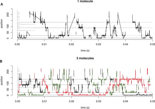
Dynamic behaviour of TF molecules. We consider a random 250 bp DNA and TF molecules which can bind/unbind, hop, jump, slide left/right. (A) 1 TF molecule (B) 3 TF molecules. The position of the molecules is represented on y-axis and the time on the x-axis. The grey line on the y-axis represents the affinity at that position for a TF. Note that after a complete dissociation of a TF from the DNA the line that follows the position is broken as opposed to a line connecting two dense regions which describes a hop or a correlated jump.

One simple test consists of plotting the normalized affinity versus the normalized occupancy for each position on the DNA after the simulator is run for a long-time interval. The top graph in Figure 3 shows that there is a strong positive correlation between occupancy-bias on the DNA and affinity, in the case of 1 TF molecule in the system.

Fig. 3.

Open in new tabDownload slide

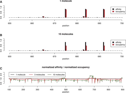
Affinity vs occupancy. We consider a random 1000 bp DNA strand and TF molecules which can bind/unbind, hop, jump, slide left/right. In (A) we show the normalized affinity and normalized occupancy for 1 molecule and in (B) for 10 molecules. In (C) we plot the ratio between occupancy and affinity, which should be ~1 for highly correlated values. The Pearson, coefficient of correlation between the the affinity and occupancy slightly drops from 0.999 (in the case of 1 molecule) to 0.998 (in the case of 3 molecules) and, further, to 0.979 (in the case of 10 molecules).

Furthermore, in the case of multiple molecules of the same TF species, the affinity and occupancy have a strong correlation, but not as good as in the case of 1 molecule (see middle plot of Fig. 3). This suggests that in the case of crowding and competition for DNA space, the affinity between TF molecules and DNA is not the sole determinant of the occupancy-bias. Inverting this statement, we could say that occupancy-bias is not necessarily equivalent to the affinity landscape, in the sense that regions that are occupied most of the time are not necessarily the highest affinity ones. However, this was observed at 1 bp resolution and it might be averaged out on larger sectors of DNA.

Finally, we would like to mention that in the Supplementary Material, we systematically investigated the quality of our approach to estimate model parameters. The results showed that setting the model parameters using our approach leads to negligible errors between the desired system behaviour and the measured one in the simulations.

5 CONSIDERATIONS ON THE MODEL

One question that one might ask is whether our coarse-grained model of 3D diffusion will capture all the details of a real 3D particle simulator. van Zon et al. (2006) observed that the zero-dimensional Chemical Master Equation can accurately model the association rate between TF molecules and the DNA, as long as the model considers fast re-binding in close proximity after an unbinding event. Since we implemented fast re-binding in our model (through hops), we conclude that the 3D diffusion model employed in this contribution reliably represents the 3D diffusion of TFs in the cytoplasm.

Furthermore, we did not consider the 3D shape of the DNA in our model. Nevertheless, the shape of the DNA is likely to affect only two variables in the model, namely: (i) the average number of re-bindings [because it is expected that once trapped in dense DNA areas, the TF molecules will find it more difficult to escape the DNA (Bancaud et al., 2009)] and (ii) the areas of the DNA where a TF will hop [hopping is more likely to lead to small 1D displacement, but in the case of close 3D proximity, this might result in more jumping (Lomholt et al., 2009)]. Both of these parameters are fine-tunable within our model, so by increasing the hopping lengths and the number of fast re-bindings, 3D effects could be integrated in the model.

In addition, we also make the assumption that the 1D random walk is unbiased. However, some previous models of sliding considered that the 1D random walk is biased, in the sense that depending on the left or right side affinities from the current position a TF molecule might have different probabilities to slide in one or the other direction (Slutsky and Mirny, 2004). This was supported by the fact that the affinity landscape of RNAp seems to increase when moving towards the transcription start site (TSS) and consequently the RNAp can be directed towards the TSS (Weindl et al., 2007).

Barbi et al. (2004) showed that in the case of bias, the random walk displays initially a sub-diffusive behaviour which can last significantly long. However, Blainey et al. (2006) did not observe any anomalous 1D diffusion when a hOgg1 protein would perform a random walk on the DNA in vitro, but rather concluded that the random walk is unbiased. Since there is no strong experimental evidence for the fact that biased random walk is a general mechanism in the search process, we considered in this contribution that the random walk is unbiased.

Finally, in comparison to a different implementation strategy, the memory model proposed by (Barnes and Chu, 2010), our implementation strategy showed an increase in speed (see Supplementary Material). The disadvantage of our strategy is that creating an array with the same size as the DNA for each TF species, will result in larger memory requirements compared with the memory model of (Barnes and Chu, 2010). For the entire genome of E.coli (4.6 Mbp) and two TF species, a non-cognate and a cognate one, the simulator will require approximately 2 GB of RAM. Although the simulator permits to specify input several species of TF, extra care should be taken when adding new species into the simulator due to the extra memory usage. Each new TF species added to this system (E.coli) will increase the required memory by a few hundred MB (≈300 MB) for a DNA sequence of 4.6 Mbp. However, we consider our strategy as a good compromise in cases were simulation speed is essential.

6 DISCUSSION

Previously, facilitated diffusion was modelled mainly analytically (e.g. Berg et al., 1981; Mirny et al., 2009). Although these types of models brought new insights into the mechanism, they mainly lack the capability to integrate real DNA sequence (a non-uiniform TF affinity ‘landscape’; Mirny et al., 2009) and/or dynamic crowding (mobile ‘roadblocks’; Flyvbjerg et al., 2006; Li et al., 2009). Nevertheless, computational models are able to surpass these shortcomings.

Stochastic simulations have revolutionized the way theoretical biologists can nowadays deal with problems that are not easily amenable to experimental measurements. TF target finding belongs to a class of spatio-temporal problems that, in a first approximation, may be addressed with tools that simulate 3D diffusion, e.g. Smoldyn (Andrews et al., 2010). However, due to the particular behaviour of DNA-binding proteins and the proposed facilitated diffusion mechanism, the Smoluchowski limit is overcome. For a meaningful outcome from any simulation experiment, a more detailed model is therefore required. In order to produce results in a relatively short time, previous computational models of facilitated diffusion were limited by size of the analyzed system or level of details included in the model. For example, the work of (Das and Kolomeisky, 2010) and (Wunderlich and Mirny, 2008) did not consider specific affinities between TF and DNA, while more detailed models as the one presented by (Chu et al., 2009) could consider at most 40 kbp per DNA strand.

Our model includes new features that were not previously considered in this type of modelling, such as TF orientation on the DNA and the fact that TF can cover more base pairs than the actual DNA binding domain. In addition, we also suggested an implementation strategy that allows for genome-size DNA sequences to be simulated, a clear advantage over previous tools there were limited to few thousands base pairs (Chu et al., 2009).

Not only does our work proposes a detailed model of the facilitated diffusion mechanism with a highly efficient implementation strategy, but also presents a systematic and comprehensive assessment of crucial parameters in this system. As an example, we use (Elf et al., 2007) measurements of the lac repressor system in E.coli. In particular, we show that using our comprehensive parameter estimation, our model displays similar behaviour as in (Elf et al., 2007), i.e. residence time of t_R=5 ms, actual sliding lengths of s_l^obs=90 bp, the relative time the molecules stays bound to the DNA of f=0.9 and the 1D diffusion coefficient of 0.046 μm²s⁻¹.

It can therefore be concluded that for future studies on TF target finding in prokaryotic systems, our model represents an ideal entry point for stochastic simulations.

ACKNOWLEDGEMENTS

We would like to thank Robert Foy and Robert Stojnic for useful discussions and comments on the manuscript.

Funding: Medical Research Council [G1002110 to N.R.Z.] and Royal Society [to B.A.].

Conflict of Interest: none declared.

REFERENCES

Author notes