


Abstract
Motivation: The estimation of species phylogenies requires multiple loci, since different loci can have different trees due to incomplete lineage sorting, modeled by the multi-species coalescent model. We recently developed a coalescent-based method, ASTRAL, which is statistically consistent under the multi-species coalescent model and which is more accurate than other coalescent-based methods on the datasets we examined. ASTRAL runs in polynomial time, by constraining the search space using a set of allowed ‘bipartitions’. Despite the limitation to allowed bipartitions, ASTRAL is statistically consistent.
Results: We present a new version of ASTRAL, which we call ASTRAL-II. We show that ASTRAL-II has substantial advantages over ASTRAL: it is faster, can analyze much larger datasets (up to 1000 species and 1000 genes) and has substantially better accuracy under some conditions. ASTRAL’s running time is , and ASTRAL-II’s running time is , where n is the number of species, k is the number of loci and X is the set of allowed bipartitions for the search space.
Availability and implementation: ASTRAL-II is available in open source at https://github.com/smirarab/ASTRAL and datasets used are available at http://www.cs.utexas.edu/~phylo/datasets/astral2/.
Contact: smirarab@gmail.com
Supplementary information: Supplementary data are available at Bioinformatics online.
1 Introduction
The estimation of species trees is complicated by the fact that different parts of the genome have different evolutionary histories; therefore, the different ‘gene trees’ obtained on different loci are often in conflict with each other and with the true species tree. Gene tree discord due to incomplete lineage sorting (ILS) is a major challenge to species tree estimation (Degnan and Rosenberg, 2009; Edwards, 2009; Maddison, 1997) and is a particular problem for rapid radiations (where several speciation events occur in a relatively short amount of time).
Because of the possibility of gene tree conflict, species tree estimations are increasingly based on multiple loci. One approach to estimating the species tree simply concatenates the sequence alignments for the different loci together and estimates a tree on the concatenated alignment. However, concatenation-based analyses can be statistically inconsistent under the multi-species coalescent (Roch and Steel, 2014) and can result in incorrect trees with high support (Kubatko and Degnan, 2007). Because of this potential for concatenation analyses to produce incorrect species trees, many methods have been developed that are designed to address gene tree incongruence due to ILS. Some of these methods have been proven statistically consistent under the multi-species coalescent (Rannala and Yang, 2003), which means that they will return the true species tree with high probability, given a large enough number of true gene trees. Some of these coalescent-based methods [e.g. MP-EST by Liu et al. (2010) and NJst by Liu and Yu (2011)] are now in widespread use.
Despite the availability of coalescent-based methods, many biological datasets are too large for the available methods; for example, MP-EST cannot be used on large datasets due to computational reasons (Bayzid et al., 2014). Other coalescent-based methods are even more limited; for example, *BEAST (Heled and Drummond, 2010), a method that co-estimates gene trees and the species tree, cannot be used with more than about 25 species (Zimmermann et al., 2014). Computational challenges in real dataset analyses have required the development of coalescent-based methods that could analyze larger datasets; for example, MP-EST could not analyze the 1KP (Wickett et al., 2014) dataset of about 100 species and 600 genes, due to the dataset size among other issues.
ASTRAL (Mirarab et al., 2014a) was developed to enable coalescent-based analyses of these larger datasets. ASTRAL solves a likely NP-hard problem by constraining the allowed search space to those species trees that derive their bipartitions from an input set X, provided by the user. In the default setting for ASTRAL, we set X to be all bipartitions in the input gene trees. ASTRAL is statistically consistent under the multi-species coalescent using this setting for X and runs in polynomial time. ASTRAL also had excellent accuracy on the datasets (both simulated and biological) that we explored in Mirarab et al. (2014a); however, all these datasets were relatively small (at most 37 species). Our subsequent evaluation of ASTRAL, which we report here, shows that ASTRAL’s running time increases quickly for large datasets and that setting X to be the bipartitions in the input gene trees reduces the accuracy for species trees estimated by ASTRAL under certain model conditions. In particular, this setting for X is a problem in the presence of large numbers of taxa, few gene trees or high levels of discordance.
We introduce ASTRAL-II, a new version of ASTRAL. We improve the running time asymptotically by a factor of n (where n is the number of species), and we show how to define the set X so that ASTRAL is more robust and also explores a larger search space. We have also modified ASTRAL so that it can handle polytomies in the input trees. We compare ASTRAL to coalescent-based species tree estimation methods and to concatenation using maximum likelihood (CA-ML) on a collection of simulated datasets and a biological dataset. We show that ASTRAL outperforms the coalescent-based methods, providing improved accuracy, and is able to analyze very large datasets. In particular, we show that ASTRAL can analyze 1000 species and 1000 genes in about a day, using a single processor. The comparison between ASTRAL and CA-ML shows that ASTRAL is more accurate whenever the ILS level is sufficiently high and comes close to CA-ML under very low ILS levels. Our extensive simulations show how the choice of the best method to use can often depend on the amount of gene tree error, number of genes and the level of discordance. On the biological data, we show that some differences between CA-ML and MP-EST previously attributed to the fact that MP-EST accounts for ILS have to be interpreted with care, because ASTRAL-II, which is also consistent under ILS, recovers topologies similar to CA-ML.
2 Background: ASTRAL-I
Given a set of k binary input gene trees on n taxa, there is a multi-set of quartet trees induced by the input. We define the weighted quartet (WQ) score of a given tree as the number of quartet trees from this multi-set that the given tree also induces. The optimization problem solved by ASTRAL is to find the species tree that maximizes the WQ score (Mirarab et al., 2014a).
Let X0 denote the set of bipartitions found in the input gene trees. If , then using ASTRAL with the set X is statistically consistent under the multi-species coalescent model.
3 ASTRAL-II
ASTRAL-II has three new features: (i) it uses a faster algorithm to compute w, (ii) it searches a larger space by expanding the set X using heuristics and (iii) it can handle polytomies in its input.
3.1 Running time improvement
The score w (Equation 2) needs to be calculated for each tripartition and such tripartitions need to be scored. ASTRAL-I computes w in time for each tripartition, but in ASTRAL-II, we use a better algorithm that uses only O(nk) time. In ASTRAL-I, we sum over O(nk) input gene tree nodes, and, for each node, we first calculate C and then compute QI using Equation (1). We represent subsets of taxa as bitsets, which results in O(n) running time for calculating C; therefore, calculating each w requires . In ASTRAL-II, instead of looking at tripartitions in input gene trees, we do a post-order traverse of all gene trees (rooted arbitrarily) and calculate the score using the algorithm shown in Algorithm 1.
function WEIGHT () and empty stack
fordo
ifu is a leaf then
else
pull from S
pull from S
push (x, y, z) to S
function GETSIMILARITY ()
for and do
fordo
fordo
function ADDBYGREEDY ()
fordo
fordo
and
whilec < maxdo
ifthen
ifthen
fordo
This algorithm, for each traversal node u, computes the number of taxa under u that are shared with each side of the tripartition being scored. This is done using a O(1) calculation that sums the same quantities already calculated for the children of u. At the leaves, we simply need to find which side of the tripartition includes that leaf, which can also be done in O(1) using bitsets. Thus, we easily compute the C matrix in O(1) and therefore, calculating w for each tripartition requires O(nk) running time. Thus,
The running time of ASTRAL-II is .
3.2 Additions to X
We use following heuristic strategies to add bipartitions to the set X.
3.2.1 Similarity matrix
We define the similarly between a pair of taxa as the number of quartet trees induced by gene trees where the pair appear on the same side of the quartet. We compute a similarity matrix by traversing all nodes of input gene trees, rooted arbitrarily (Algorithm 2). For each node u, we look at all pairs of leaves chosen each from one of the children of u. For each such pair, we add to their similarity score, where y is the number of leaves outside the subtree below u. This will process each pair of nodes in each of the input k genes exactly once and would therefore require computations. The final score can be normalized by the number of input quartet trees that include any pair (not shown in Algorithm 2). We use the similarity matrix to calculate a UPGMA tree and add all its bipartitions to X. This matrix is also used in our next heuristics.
3.2.2 Greedy
The greedy consensus of a set of trees is obtained by starting from a star tree and adding bipartitions from input trees in the decreasing order of their frequency if they do not conflict with previous bipartitions. This process ends when no remaining bipartition has frequency above a given threshold or when the tree is fully resolved. We estimate the greedy consensus of the gene trees with various thresholds (Algorithm 3). For each polytomy in each consensus tree, we resolve the polytomy in multiple ways and add bipartitions implied by those resolutions to the set X. First, we resolve the polytomy by applying UPGMA to the similarity matrix, starting from clusters defined by the polytomy. Then, we sample one taxon from each side of the polytomy randomly and use the greedy consensus of the gene trees restricted to this subsample to find a resolution of the polytomy (randomly resolving remaining polytomies). We repeat this process at least 10 times, but if the subsampled greedy consensus trees include new bipartitions that are sufficiently frequent (), we do more rounds of random sampling (we increase the number of iterations by two). For each random subsample around a polytomy, we also resolve it by calculating an UPGMA tree on the subsampled similarity matrix. Finally, for the two first greedy threshold values and the first 10 random subsamples, we also use a third strategy that can potentially add a larger number of bipartitions: for each subsampled taxon x, we resolve the polytomy as a pectinate tree by sorting the remaining taxa according to their similarity with x (in decreasing order).
3.2.3 Gene tree polytomies
When gene trees include polytomies, we also add new bipartitions to set X. We first compute the greedy consensus of the input gene trees with threshold 0, and if the greedy consensus has polytomies, we resolve them using UPGMA; we repeat this process twice to account for random tie-breakers in the greedy consensus estimation. Then, for each gene tree polytomy, we use the two resolved greedy consensus trees to infer a resolution of the polytomy, and we add the implied resolutions to set X.
3.3 Multifurcating input gene trees
In the presence of polytomies, the running time analysis can change because analyzing each polytomy requires time cubic in its degree and the degree can increase with n. It is not hard to see that the worst case is when all gene trees have a polytomy with ; in this case, the running time is .
3.4 Statistical consistency
Theorem 3
ASTRAL-II is statistically consistent under the multi-species coalescent model.
Proof
The changes made to ASTRAL-I to develop ASTRAL-II affect the running time, enlarge the search space and allow it to analyze gene trees with polytomies. Under the multi-species coalescent model, all gene trees are binary. As shown in Theorem 1, as long as the set X contains all the bipartitions in the input gene trees, ASTRAL is statistically consistent. The theorem follows.
4 Experimental setup
4.1 Simulation procedure
We used SimPhy (https://github.com/adamallo/SimPhy) to simulate species trees and gene trees (produced in mutation units) and then used Indelible (Fletcher and Yang, 2009) to simulate nucleotide sequences down the gene trees with varying length and model parameters. We estimated gene trees on these simulated gene alignments, which we then used in coalescent-based analyses.
We simulated 11 model conditions, which we divide into two datasets, with one model condition appearing in both datasets. We used SimPhy to simulate species trees according to the Yule process, characterized by the number of taxa, maximum tree length and the speciation rate (this combination defines a model condition). In six model conditions (forming Dataset I), we fixed the number of taxa to 200 and varied tree length (500 K, 2 M and 10 M generations) and speciation rates (1e-6 and 1e-7 per generation). The tree length impacts the amount of ILS, with lower length resulting in shorter branches, and therefore higher levels of ILS (Supplementary Fig. 1a). Speciation rate impacts whether speciation events tend to happen close to the tips (1e-06) or close to the base (1e-07). Different tree shapes (i.e. combinations of tree length and speciation rate) produce different levels of ILS starting from relatively low [roughly 10% distance between true gene trees and the species tree, measured by the Robinson–Foulds (RF) distance; Robinson and Foulds (1981)] and going up to very high (roughly 70% RF). In the remaining model conditions (forming Dataset II), we fixed the tree shape to 2 M/1e-06 and set the number of taxa to 10, 50, 100, 200, 500 and 1000. Thus, the model condition with 200 taxa and the 2 M/1e-6 tree shape appears in both datasets.
For each model condition, we simulated 50 species trees, forming 50 replicates. On each species tree, 1000 gene trees were simulated according to the multi-species coalescent model with the population size fixed to 200 000 (a reasonable value for vertebrates). SimPhy uses various rate parameters and rate heterogeneity modifiers to convert gene tree branch lengths to mutation units, introducing deviations from molecular clock and rate heterogeneity between genes (see Supplementary Table S1 for parameters; simulation scripts available at http://www.cs.utexas.edu/users/phylo/software/astral/).
We simulated indel-free gene alignments using Indelible and under the GTR + Γ model. First, for each replicate, two parameters, μ and σ, were drawn uniformly from and respectively. Then, the sequence length for each gene in that replicate was drawn from a log-normal distribution with μ and σ parameters (thus, average sequence length is uniformly distributed between 300 bp and 1500 bp). GTR + Γ parameters were drawn from Dirichlet distributions that had parameters estimated using ML from a collection of real biological datasets (details given in the Supplementary Material).
4.2 Gene tree estimation
Previous studies (Liu et al., 2011) have shown that FastTree-II (Price et al., 2010) is generally as accurate at estimating the tree topology as more extensive ML heuristics such as RAxML (Stamatakis 2014), while being much faster. In our simulation studies, we used FastTree to estimate the 550 000 gene trees ranging from 10 to 1000 species. Figure 1b shows the distribution of gene tree estimation error and demonstrate that we have simulated wide-ranging levels of gene tree error. The tree error was impacted by tree shape parameters; more ILS and deeper speciation lead to higher levels of gene tree error. Moreover, average gene tree estimation error varied across replicates, and gene tree error varied considerably among the 1000 genes in each replicate; the number of taxa had only a small impact on gene tree estimation error (Supplementary Fig. S1).
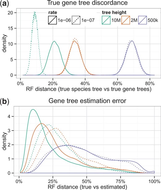
Characteristics of the simulation. (a) RF distance between the true species tree and the true gene trees (50 replicates of 1000 genes) for Dataset I. Tree height directly affects the amount of true discordance; the speciation rate affects true gene tree discordance only with 10 M tree length. The number of taxa has a modest effect on the discordance (see Supplementary Fig. S13). (b) RF distance between true gene trees and estimated gene trees for Dataset I. See also Supplementary Figure S1 for inter- and intra-replicate gene tree error distributions
FastTree can output polytomies when sequence alignments cannot distinguish between competing tree resolutions. We removed any gene tree where more than 50% of the internal nodes were polytomies. This pruning left fewer than 500 genes for three replicates of the 200 taxon/500 K/1e-06 and 50-taxon model conditions, two replicates of the 100-taxon model condition and one replicate of the 10-taxon model condition. Those nine replicates (out of 550) were removed from our analyses.
4.3 Species tree methods
We run all methods given a maximum of 4 days of running time and 24 GB of memory. We compare ASTRAL-I to ASTRAL-II and ASTRAL-II to NJst and CA-ML run using FastTree. MP-EST only finished for datasets with at most 100 taxa within time limits. Because of its running time, we ran MP-EST once (one random seed number) for each analysis. NJst, ASTRAL-I and MP-EST could not handle polytomies; therefore, we randomly resolved polytomies in inputs of these methods. We also ran ASTRAL-II on gene trees with randomly resolved polytomies and observed no differences with ASTRAL-II run on gene trees with polytomies (Supplementary Fig. S12). Thus, differences between ASTRAL-II and other methods are not due to the random resolutions of polytomies.
4.4 Evaluation criteria
We evaluate methods in terms of species tree error and we also evaluate running time for coalescent-based methods. Species tree error is measured using the standard RF distance. Running time of summary methods is measured on a heterogeneous condor cluster and gives the wall clock running time.
5 Simulation results
We start by comparing ASTRAL-II with ASTRAL-I in terms of accuracy and running time (RQ1). We next focus on ASTRAL-II and compare it to other coalescent-based methods (RQ2) and then compare it to CA-ML (RQ3). This question leads us to a more in depth analysis of the effects of gene tree estimation error on the accuracy of various methods (RQ4). Finally, we evaluate the impact of collapsing low support branches in input gene trees on the accuracy of ASTRAL-II (RQ5).
5.1 RQ1: ASTRAL-I versus ASTRAL-II
5.1.1 Search space
ASTRAL-II adds extra bipartitions to the search space, which allows it to explore a larger search space; this tends to increase the accuracy of ASTRAL-II over ASTRAL-I. In our simulations, the extent of the improvement depended on the model condition (Table 1). In Dataset I, with the lowest level of ILS or with the medium ILS level and recent speciation, both ASTRAL-I and ASTRAL-II had extremely low error (Supplementary Fig. S2) and no substantial improvements were detected by the addition of extra bipartitions (Table 1). With 2M length and deep speciations, ASTRAL-II improved upon ASTRAL-I substantially, with improvements ranging from 3.5% with 1000 genes to 10.1% with 50 genes. Most dramatic differences were observed on the high ILS conditions, where ASTRAL-I performed extremely poorly (Supplementary Fig. S2), but ASTRAL-II reduced the error by about 40% (Table 1). Results on Dataset II showed that the effect of adding extra bipartitions also depended on the number of taxa in expected ways (Table 1). With this fixed tree shape, ASTRAL-I was as accurate as ASTRAL-II for up to 200 taxa, but with 500 taxa or more, ASTRAL-II had a substantial advantage (as large as 9%). As expected, the advantage of ASTRAL-II was larger with few genes and reduced with more genes.
Reductions in species tree error obtained by ASTRAL-II compared with ASTRAL-I
| Dataset I [200 taxa, varying tree shape (columns) and number of genes (rows)] | ||||||
|---|---|---|---|---|---|---|
| 10e-6 (recent) | 10e-7 (deep) | |||||
| 10 M | 2 M | 500 K | 10 M | 2 M | 500 K | |
| 50 | 0.2 ± 0.2 | 0.7 ± 0.3 | 37.9 ± 1.0 | 1.7 ± 0.6 | 10.1 ± 0.9 | 38.7 ± 0.9 |
| 200 | 0.0 ± 0.1 | 0.2 ± 0.1 | 41.0 ± 1.1 | 0.7 ± 0.3 | 7.4 ± 0.7 | 41.4 ± 1.0 |
| 1000 | 0.0 ± 0.0 | 0.2 ± 0.1 | 39.2 ± 1.2 | 0.0 ± 0.0 | 3.5 ± 0.7 | 41.4 ± 1.1 |
| Dataset II [2M/1e-6 shape, varying the number of taxa (columns) and genes (rows)] | ||||||
| 10 | 50 | 100 | 200 | 500 | 1000 | |
| 50 | 0.3 ± 0.3 | 0.0 ± 0.1 | 0.3 ± 0.2 | 0.7 ± 0.3 | 6.0 ± 0.6 | 9.3 ± 0.6 |
| 200 | 0.0 ± 0.0 | 0.0 ± 0.0 | 0.0 ± 0.0 | 0.2 ± 0.09 | 3.9 ± 0.5 | 8.3 ± 0.5 |
| 1000 | 0.0 ± 0.0 | 0.1 ± 0.1 | 0.0 ± 0.0 | 0.2 ± 0.08 | 1.7 ± 0.4 | |
We report results using the difference in RF percentage; values above 0.0% indicate ASTRAL-II is more accurate.
The improvements obtained by ASTRAL-II are due to additions to the search space. We therefore asked whether the heuristic approaches used to add bipartitions to set X are sufficient or improvements could be obtained by further expanding X. To answer this question, we tested the impact of adding all the bipartitions from the species tree to the set X and compared ASTRAL-II with and without these extra bipartitions (see Supplementary Figs S2 and Supplementary Data). We saw no significant differences between ASTRAL-II with and without these potentially new bipartitions (P = 0.77 according to a two-way analysis of variance test), indicating that the accuracy of ASTRAL-II is very unlikely to be improved further by expanding the search space.
5.1.2 Running time
With 200 taxa and lower levels of ILS, ASTRAL-I and ASTRAL-II had similar running times (Supplementary Fig. S2), but ASTRAL-II was faster with increased ILS (3 versus 7.5 h of median run time). Note that ASTRAL-II searches a larger tree space than ASTRAL-I. With small numbers of taxa, the two versions had close running times, but as the number of taxa increased, the running time of ASTRAL-II increased more slowly (Supplementary Fig. S3). For 500 taxa, ASTRAL-II was twice as fast as ASTRAL-I (a median of 5 versus 10 h), whereas ASTRAL-I did not complete on 1000 taxa and 1000 genes.
5.2 RQ2: ASTRAL-II versus other coalescent methods
We refer to ASTRAL-II as ASTRAL henceforth.
Completion within time constraints ASTRAL completed on all model conditions, MP-EST completed only on datasets with at most 100 taxa and NJst completed on all model conditions except for the condition with 1000 genes and 1000 taxa.
Dataset I ASTRAL was more accurate than NJst in all model conditions, except 1e-07/500 K where the two methods had identical accuracy (Fig. 2). Overall, the differences between ASTRAL-II and NJst were statistically significant (), according to a two-way analysis of variance test, and the relative performance of the methods was significantly impacted by the speciation rate (P = 0.026) but not by the number of genes or tree length. ASTRAL was faster than NJst, in some cases by an order of magnitude and in other cases by smaller margins (Supplementary Fig. S4).
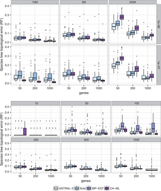
Comparison of methods with respect to species tree topological accuracy. (Top) Two hundred taxa and varying tree shapes and number of genes. (Bottom) Varying number of taxa and genes and tree shaped fixed to 2 M/1e-6. ASTRAL-II is always at least as accurate as NJst and MP-EST
Dataset II On 10-taxon datasets, all methods had high accuracy (Supplementary Table S2). On 50- and 100-taxon datasets, MP-EST was able to finish, but it was the least accurate of all the methods. ASTRAL was more accurate than NJst for all conditions except for 50 taxa with 50 genes (Supplementary Table S2); however, differences were generally small when the number of taxa was 200 or less and more substantial with more taxa. Overall, differences between ASTRAL and NJst were significant (P = 0.0007) and were significantly impacted by the number of taxa (P = 0.0004) but not the number of genes. ASTRAL was also faster than NJst, especially with more genes and more taxa (Fig. 3). For example, on 500 taxa and 1000 genes, ASTRAL typically finished in 2–10 h, whereas NJst required 12–30 h (Supplementary Fig. S5). MP-EST was by far the slowest method, but its running time was not impacted by the number of genes.
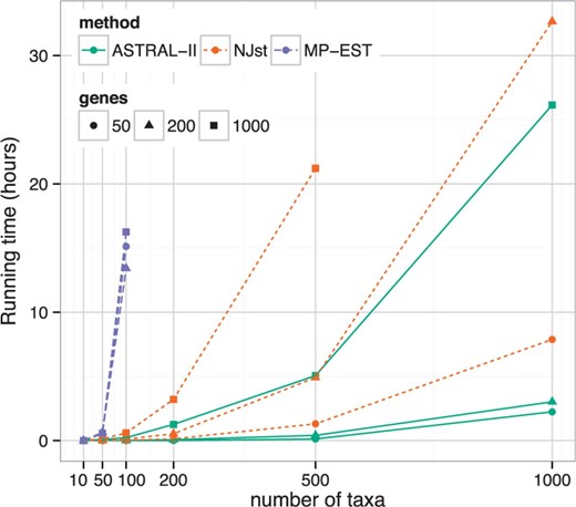
Running time comparison with varying number of taxa and genes (Dataset II). Average running time is shown for NJst and ASTRAL-II. Note that ASTRAL-II is much faster on large datasets
5.3 RQ3: ASTRAL-II versus CA-ML
5.3.1 Dataset I
Interestingly, the relative accuracy of CA-ML and ASTRAL was significantly impacted by tree length (), speciation rate (P = 0.00004) and the number of genes (). With lower levels of ILS (10M and 2 M) and recent speciation, CA-ML and ASTRAL had close accuracy, but CA-ML tended to be better with more genes and ASTRAL was better with fewer genes (Supplementary Table S1, Fig. 2). With deep speciation and lower ILS, CA-ML was substantially more accurate than ASTRAL, but increasing the number of genes reduced the gap. At the high ILS levels, ASTRAL was much more accurate than CA-ML for all number of genes and for both recent and deep speciation.
5.3.2 Dataset II
Overall, differences between ASTRAL and CA-ML were not significant (P = 0.2), but the relative accuracy seemed to be impacted by the number of genes (P = 0.06). Regardless of the number of taxa, which did not impact relative accuracy (P = 0.2), CA-ML was slightly more accurate with 1000 genes and ASTRAL was slightly more accurate with fewer genes (Supplementary Table S2, Fig. 2).
5.3.3 Running time
We ran CA-ML and ASTRAL-II on different platforms and hence cannot make direct running time comparisons. Nevertheless, we provide our running time numbers to give a general idea. CA-ML using FastTree on 200-taxon model conditions with 1000 genes took roughly 2 h, whereas ASTRAL-II took roughly one hour to estimate the species tree and estimating gene trees also took about 1.5 h. In general, therefore, the running times of ASTRAL-II and CA-ML are relatively close on this dataset.
5.4 RQ4: effect of gene tree error
In RQ3, we observed that under some conditions, CA-ML was more accurate than ASTRAL, a pattern that we attribute to high levels of gene tree error present in our simulations. When true (simulated) gene trees are used instead of the estimated gene trees, the accuracy of ASTRAL is outstanding, regardless of the model condition (see Fig. 4 and Supplementary Fig. S6), and ASTRAL is always more accurate than CA-ML. Thus, the fact that CA-ML is more accurate than ASTRAL under lower levels of ILS is related to estimation error in the input provided to ASTRAL.
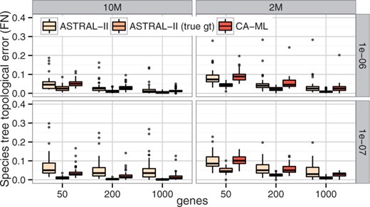
Comparison of ASTRAL-II run using estimated and true gene trees and CA-ML on Dataset I
In our ASTRAL and NJst analyses, gene tree error had a positive correlation with species tree error (Supplementary Fig. S7), with correlation coefficients that were similar for ASTRAL and NJst. The error of CA-ML also correlated with gene tree error (obviously the relationship is indirect; for example, short alignments impact both CA-ML and gene tree error), but the correlation was weaker than the correlation observed for coalescent-based methods (Supplementary Fig. S8). Interestingly, the correlation between gene tree estimation error and species tree error was typically higher with fewer genes.
To further investigate the impact of the gene tree error, we divided replicates of each model condition into three categories: average gene tree estimation error below 0.25 is low, between 0.25 and 0.4 is medium and above 0.4 is high. We plotted the species tree accuracy within each of these categories (see Fig. 5 for one model condition, but also see Supplementary Figs S9 and Supplementary Data for other model conditions). The relative performance of ASTRAL and NJst is typically unchanged across various categories of gene tree error, but increasing gene tree error tends to increase the magnitude of the difference between ASTRAL and NJst. Furthermore, MP-EST seemed to be more sensitive to gene tree error than either NJst or ASTRAL (Supplementary Fig. S10).
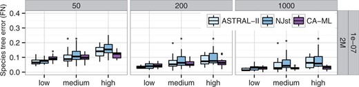
Comparison of species tree accuracy with 200 taxa, divided into three categories of gene tree estimation error. Boxes show number of genes
The relative performance of ASTRAL and CA-ML depended on gene tree error. For those model conditions where CA-ML was generally more accurate than ASTRAL (e.g. 2 M/1e-07), ASTRAL tended to outperform CA-ML on the replicates with low gene tree estimation error (Fig. 5). Consistent with this observation, we noted that ASTRAL was impacted by gene tree error more than CA-ML (Supplementary Fig. S9).
5.5 RQ5: collapsing low support branches
ASTRAL-II can handle inputs with polytomies. Although we have not done bootstrapping to get reliable measures of support, we do get local SH-like branch support from FastTree-II. We collapsed low support branches (10%, 33% and 50%) and ran ASTRAL on the resulting unresolved gene trees. We measured the impact of contracting low support branches on the RF rate: the median delta RF (error before collapsing minus error after collapsing) is typically zero (Supplementary Fig. S11), never above zero but in a few cases below zero (signifying that accuracy was improved in those few cases). However, these differences are not statistically significant (P = 0.36). Since this analysis was performed using SH-like branch support values instead of bootstrap support values (or other ways of estimating support values), further studies are needed.
6 Biological results
The evolution of angiosperms, and the placement of Amborella trichopoda Baill., is one of the challenging questions in land plant evolution. One hypothesis recovered in some recent molecular studies (e.g. Drew et al. 2014; Qiu et al. 2000; Wickett et al. 2014; Zhang et al. 2012) is that A.trichopoda Baill. is sister to the rest of angiosperms, followed by water lilies (i.e. Nymphaeales). In particular, a recent analysis of 104 plant species based on entire transcriptomes recovered this relationship both with concatenation and ASTRAL-I, using various perturbations of the dataset (Wickett et al., 2014). A competing hypothesis is that Amborella is sister to water lilies, and this whole group is sister to other angiosperms (Drew et al., 2014; Goremykin et al., 2013). Xi et al. (2014) examined this question using a collection of 310 genes sampled from 42 angiosperms and 4 outgroups. They observed that CA-ML produced the first hypothesis and MP-EST produced the second hypothesis, and they argued that these differences are due to the fact that CA-ML does not model ILS, whereas MP-EST does.
We obtained alignments for these 310 genes from Xi et al. (2014) and estimated gene trees using RAxML under GTR + Γ model with 200 replicates of bootstrapping and 10 rounds of ML (RAxML was used because running time was not an issue on this relatively small dataset). We ran MP-EST and ASTRAL and obtained two different trees (Fig. 6). Reproducing Xi et al. (2014) results, MP-EST recovered the sister relationship of Amborella and Nymphaeales with 100% support. However, ASTRAL, just like CA-ML, recovers Amborella as sister to other angiosperms, with 75% support. Although the exact position of Amborella is debated, our analysis shows that the differences between CA-ML and MP-EST results cannot be simply attributed to the fact that CA-ML does not consider ILS.
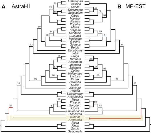
Comparison of species trees computed on the angiosperm dataset of Xi et al. (2014). MP-EST and ASTRAL-II differ in the placement of Amborella; the concatenation tree agrees with ASTRAL-II
7 Discussion and conclusion
Our wide-ranging simulation results show that ASTRAL-II, unlike the other methods we studied, can analyze datasets with up to 1000 taxa and 1000 genes within reasonable running times. However, future studies need to compare ASTRAL-II to divide-and-conquer approaches (e.g. Bayzid et al., 2014; Zimmermann et al., 2014) that enable slower coalescent-based methods to scale to large datasets. ASTRAL-II was more accurate than other coalescent-based methods and was more accurate than CA-ML, unless ILS levels were low and gene tree error was high. Although the angiosperm biological dataset we studied was relatively small (46 species), our simulations show that upcoming multi-gene datasets with large numbers of species can be accurately analyzed using ASTRAL-II.
On the angiosperm dataset, ASTRAL recovered the relationship supported by CA-ML and a large number of recent studies, whereas MP-EST recovered an alternative topology, also supported by some previous analyses. There are several possible reasons for the differences between the two methods, including the possibility that rooting gene trees (required by MP-EST but not by ASTRAL) by Selaginella can be problematic for some genes or that the impact of the gene tree estimation error is different for the two methods. We also note that ASTRAL is a non-parametric method that does not estimate branch lengths, and it is possible that non-parametric methods are less sensitive to gene tree estimation error than parametric methods (like MP-EST).
ASTRAL was more accurate than CA-ML, except when gene tree estimation error was high and ILS levels sufficiently low. These results suggest that CA-ML should not be rejected, even though it is not statistically consistent under the multi-species coalescent model. Conversely, proofs of consistency of standard summary methods assume gene trees estimated without error (Roch and Warnow, 2015), and this assumption limits the relevance of consistency results in practice. Improving gene tree estimation is crucial for coalescent-based species tree estimation, as observed in the literature (e.g. Mirarab et al. 2014b, c; Patel et al. 2013); however, the requirement to use recombination-free regions complicates this pursuit as recombination-free ‘c-genes’ can be very short, especially with increased numbers of taxa (Gatesy and Springer, 2014). Future studies need to study the impact of using shorter gene sequence alignments, and conversely the presence of recombination events within genes, used as input to coalescent-based species tree estimation methods.
Acknowledgement
We thank the anonymous reviewers for their helpful suggestions.
Funding
This work was supported by the National Science Foundation [0733029, 1461364, and 1062335 (to T.W.)]; and by a Howard Hughes Medical Institute (HHMI) graduate student fellowship (to S.M.).
Conflict of Interest: none declared.
References

